2D Patched Conics with Optional SOI Smoothing

This is a highly technical post, but I hope it helps anyone in a similar situation.

I was thinking about how to handle delta-V and timetables for orbital transfers. Originally I had planned to make up some “rules of thumb” that would provide some structure, but coming up with something that would make plausible flight times and fuel requirements sounded difficult in practice. It wasn’t long until I decided it would be easier to just… learn how to compute orbital dynamics. I wouldn’t need to deal with anything but coplanar orbits, so it couldn’t be that bad, could it? And it would be good to work it out early on since it’d be needed later for Phase One and Two anyway.

Cue 4 weeks of excitement and frustration :)

First, if you want to follow in my footsteps, be wary of some websites. There’s one in particular you should avoid altogether. I won’t link it or name it, since I don’t want to give them traffic, but I found it very misleading and the source of a lot of headache. After some digging, I found out the author works on LLM integration for the defense industry. I can’t say for sure it’s an LLM generated site, but it very confidently explains some procedures I found to be unnecessary, and I caught at least two formulae that are outright incorrect or hallucinated. You will be much better off to acquire a copy of Fundamentals of Astrodynamics by Roger R. Bate et al, published by Dover. It’s old, but celestial mechanics haven’t changed since Newton and Kepler, so it’s still a great introductory text. I was able to fill in the rest of what I needed to know with Wikipedia and Stackoverflow (the latter being less helpful than the former).

I’m not going to explain all the astrodynamics concepts, except where I struggled to find good information. This writeup focuses on how I implemented them in Godot.

Note that I resorted to compiling Godot with double precision vectors enabled. In retrospect this was not necessary for the Erua/Moon system, but over interplanetary distances the floating point errors will become significant. Depending on scope you may be fine with 32-bit vectors.

Newtonian Physics are Easy in Godot

I was able to make a 2-body Newtonian physics simulation in less than an hour, using Vector3’s and built-in vector math. To make a realistic enough simulation, you will need to determine the gravitational parameters of your celestial bodies, and determine the size of the sphere of influence (I used the Lambert sphere). Since the Erua/Moon system is an analog to Earth/Moon, I simply used the same parameters for μ and the Moon’s altitude. This gives us:

var erua_mu = 398600000000000.0

var moon_mu = 4902800000000.0

var moon_altituide = 381624236.0

var moon_soi = 65705090.504

Erua’s SOI is essentially infinite for this simulation since interplanetary trajectories are out-of-scope. Due to Godot’s draw distance limitations I scaled everything down 1000000:1, this requires conversions at certain steps.

Now, consider the state vectors r and v. These could be represented with Vector2 objects, though the h vector is perpendicular to the orbit plane, so it’s better to use Vector3 objects. These also allow for the cross product necessary to convert between state vector and Keplerian orbital elements.

So, you can suppose a spaceship orbiting between the two celestial objects. Give it some lateral velocity and account for gravity, and you can simulate its orbit. Gravity is simply a vector pointing from the ship to the main body it is orbiting, with a magnitude equal to the inverse square of the distance times the gravitational parameter of the main body. Imagine a starting velocity of 7800m/s and an altitude of 200km, and you can approximate a circular orbit. The exact velocity can be computed with the vis-viva equation. From the initial state, the gravitational force vector will be added to the spaceship’s v vector, which will be added to the position vector r with each subsequent simulation tick.

Using spheres of influence, you only need to worry about one gravity vector at a time. You could easily compute and apply both vector at all times, thus implementing n-body phyisics. However, the two-body implementation can be checked against the trajectories found in the patched conics simulation. This was helpful for debugging, at least.

Simulating an Encounter with the Moon

It is easy to approximate the Moon’s orbit by instantiating an object and placing it on a pivot centered on the main body Erua/Earth. You can then rotate the pivot by a small amount m which is the angle the Moon moves per each simulation tick. The formula for this is:

TAU / ((TAU * moon_altitude) / moon_velocity)

The Moon’s velocity can be determined with the vis-viva equation, though it is about 1021m/s. The value m corresponds to the true anomaly angle nu rather than a vector or distance.

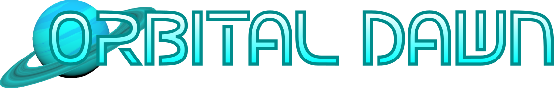
Given the Moon at an altitude of 381624236 meters, and an SOI of 65705090 meters, it is easy to simulate a spacecraft encountering the Moon. Starting with a parking orbit at 500km, it will require a velocity of 10675 m/s to make a Hohmann transfer orbit. A phase angle between 45 and 65 degrees will get the spaceship to the Moon’s SOI. For a free-return trajectory, the altitude will be a little higher and launch a little sooner than a perfect Hohmann transfer.

Considering n-body physics however, the Moon’s gravitational pull will be significant even some ways outside of its SOI. This will account for some discrepancy when simulating using conic sections. More on that later.

Given some understanding of the Newtonian simulation, we can move on to using patched conics.

Why Patched Conics?

A Newtonian simulation potentially uses a lot of computation cycles to attain the necessary fidelity to model eg. very fast speeds. Conic sections, however, are reasonable approximations of celestial mechanics, and the equations concerning them can be computed at arbitrary points in time, without simulating steps in between. Even accounting for using the Newton-Raphson method, far fewer simulation steps are required.

The drawback is accuracy, specifically at the “patch points”. Patched conics assumes the velocity vectors involved are parallel, so there will be some anomaly when crossing SOI boundaries. Compensating for this is A Problem, for which there are practical solutions, though there is no single established method.

Drawing Circles, Ellipses and Hyperbolas in 3D

Patched conics majorly deals with three of the four conic sections, being the circle, the ellipse and the hyperbola. The parabola, having an eccentricity of exactly 1, is highly unlikely to come up in practice and may be politely ignored (to paraphrase another writer). I have an ideosyncratic way of moving objects around, using “pivot” nodes to assist with circular motion i.e. attach the object you want to move to the pivot, then rotate the pivot as needed to move the object. The object can be reparented to the main scene or to other pivot nodes as needed. This method lends pretty well to moving along conic sections, since the equations all work with angles and radii.

So consider moving a spaceship model attached to a pivot, and varying its distance from the pivot based on the formulae for the three conic sections.

The Circle

This is the easiest shape to make and has already been approximated for the Newtonian simulation. It is also easy to derive the state vectors from its position and velocity: the r vector points from the orbiting object to the main body, and the v vector is always perpendicular to it.

The Ellipse

The ellipse is more difficult, but it just requires the correct equations. The equation to determine the radius of an object at a particular true anomaly is:

radius = semi_major_axis * ((1 - eccentricity ** 2) / (1 + eccentricity * cos(true_anomaly)))

Sweeping the true anomaly through 360 degrees will draw the ellipse.

The Hyperbola

Analogous to the ellipse, the equation for the radius of a hyperbola is:

radius = (h**2/mu) * (1 / (1+eccentricity*cos(true_anomaly)))

Here, h is the magnitude of the specific angular momentum of the object. It is interesting to note that hyperbolic angles are different from those of circles and ellipses, they only represent about half of the same rotation. This misled me at first, making me think there was something wrong with the equation to determine the true anomaly from the state vector. If the correct equations are used you should be able to treat them the same as any other angles.

Drawing the hyperbola will draw both the real orbit and the virtual orbit.

Now that we can draw the various conic sections, we can consider using them for orbital simulation.

The Conic Sections as a Function of Time

This is a difficult topic and I will only cover the steps I took to solve it in Godot. A more detailed explanation can be found in Fundamentals of Astrodynamics or in bits and pieces on Wikipedia.

Given True Anomaly, Find the Time of Flight

This is the “easy” side of the equation, since the solutions to Kepler’s equations are scalar.

For the ellipse: Take the given true anomaly, convert it to the eccentric anomaly, then apply Kepler’s equation to convert it to the mean anomaly, and from there the time of flight can be computed:

The eccentric anomaly: 2 * atan(sqrt((eccentricity-1)/(eccentricity+1)) * tan(true_anopmaly/2))

Mean anomaly: ecc_anomaly - eccentricity * sin(ecc_anomaly)

Time of flight: mean_anomaly * sqrt(-semi_major_axis**3/mu)

For the hyperbola: Similar, but using an analogous version of Kepler’s equation, and the hyperbolic trigonometric functions. In this case we use the hyperbolic eccentric anomaly, which is usually presented as H or F (I prefer F):

Hyperbolic eccentric anomaly: 2 * atanh(sqrt((eccentricity-1)/(eccentricity+1)) * tan(true_anomaly/2))

Mean anomaly: eccentricity * sinh(ecc_anomaly) - ecc_anomaly

Time of flight: mean_anomaly * sqrt(-semi_major_axis**3/mu)

The bad website supplies a very different formula for calculating the hyperbolic time of flight. This tripped me up for a long time before I found the correct one on Wikipedia and cross referenced with Fundamentals of Astrodynamics.

Given Time of Flight, find True Anomaly

This is more difficult, because the reverse of Kepler’s equation is trancendental. However, it can be approximated using the Newton-Raphson method of finding roots. I did this using lambdas, consider:

func solve_kepler(e, M):
    var f = func(E): return E - e*sin(E) - M
    var E = 1
    var epsilon = float(.0000001)`

## Newton's method
    while (abs(f.call(E)) > epsilon):
        E -= f.call(E)/(1 - e * cos(E))
    return E


func solve_keplerh(e, M):
    var f = func(F): return e * sinh(F) - F - M
    var F = 1
    var epsilon = float(.0000001)
    
## Newton's method
while (abs(f.call(F)) > epsilon):
	F -= f.call(F)/(e * cosh(F) - 1)
return F

For the inputs, e is the eccentricity and M is the mean anomaly. These will return the eccentric anomaly E and the hyperbolic eccentric anomaly F, respectively.

Take the given time of flight, convert to the mean anomaly, use the Newton-Raphson method to find the eccentric anomaly, and then convert to the true anomaly. Simple as!

Finding the ship’s angle at a particular time of flight is essential for placing it on the ellipse/hyperbola at the correct time.

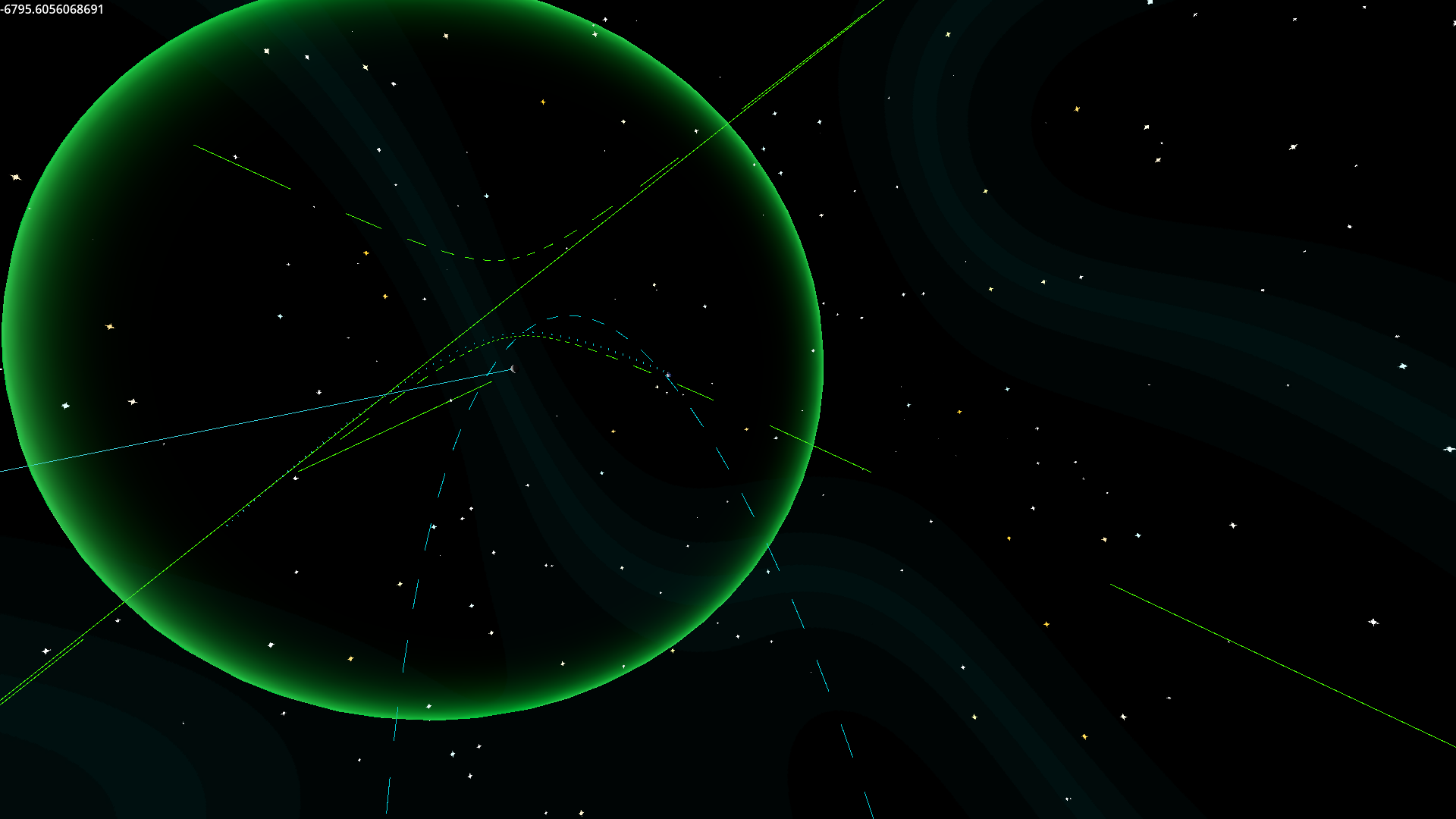
Patching Conics

Consider a spaceship crossing into the sphere of influence of a moon. Once it crosses over, we no longer care about its position and velocity vectors relative to the planet. We need to convert them to the local space. To do so, simply subtract the moon’s velocity and position vectors from the spaceship’s vectors. This is also called the hyperbolic excess velocity vector, v_inf.

(I really hope this helps someone, I had a very hard time figuring it out due to misinformation and not having the correct velocity vectors. It’s so simple in retrospect, if you understand vector math a little.)

Once you have the new r and v vectors, you can compute the h vector, thus the eccentricity vector, thus the eccentricity, thus the true anomaly. Combined with the semi-major-axis, you can find the shape of the new conic section.

With my method of drawing conics, place a pivot at the center of the moon and have it face the spacecraft. Then, rotate it by the computed true anomaly. Save this rotation (quaternion). Then, on each subsequent simulation tick, move it to the saved quaternion and then rotate it by the new true anomaly. Hope this makes sense!

Getting the State Vectors

I found it mostly sufficient to find the state vectors at the SOI crossing by pulling them from the difference in world space coordinates from the last simulation tick. That said, they can also be derived through trigonometry. Here’s the code I used:

var ship_p = ship_h**2 / erua_mu ## Semi-latus rectum
var ship_Rvec = Vector3(ship_r*sin(ship_nu),0,ship_r*cos(ship_nu))
var ship_rdotmag = sqrt(erua_mu/ship_p) * ship_e * sin(ship_nu) ## Magnitude of r-dot vector
var ship_rvdotmag = sqrt(erua_mu/ship_p) * (1 + ship_e * cos(ship_nu)) ## Magnitude of r*v-dot vector
ship_Vvec = Vector3(ship_rdotmag*sin(ship_nu)+ship_rvdotmag*cos(ship_nu),0,ship_rdotmag*cos(ship_nu)-ship_rvdotmag*sin(ship_nu))
moon_Rvec = Vector3(moon_radius*sin(moon_nu),0,moon_radius*cos(moon_nu))
moon_Vvec = moon_Rvec.normalized().rotated(Vector3(0,1,0), PI/2) * moon_v

This method is found in Fundamentals of Astrodynamics.

Optional SOI Smoothing

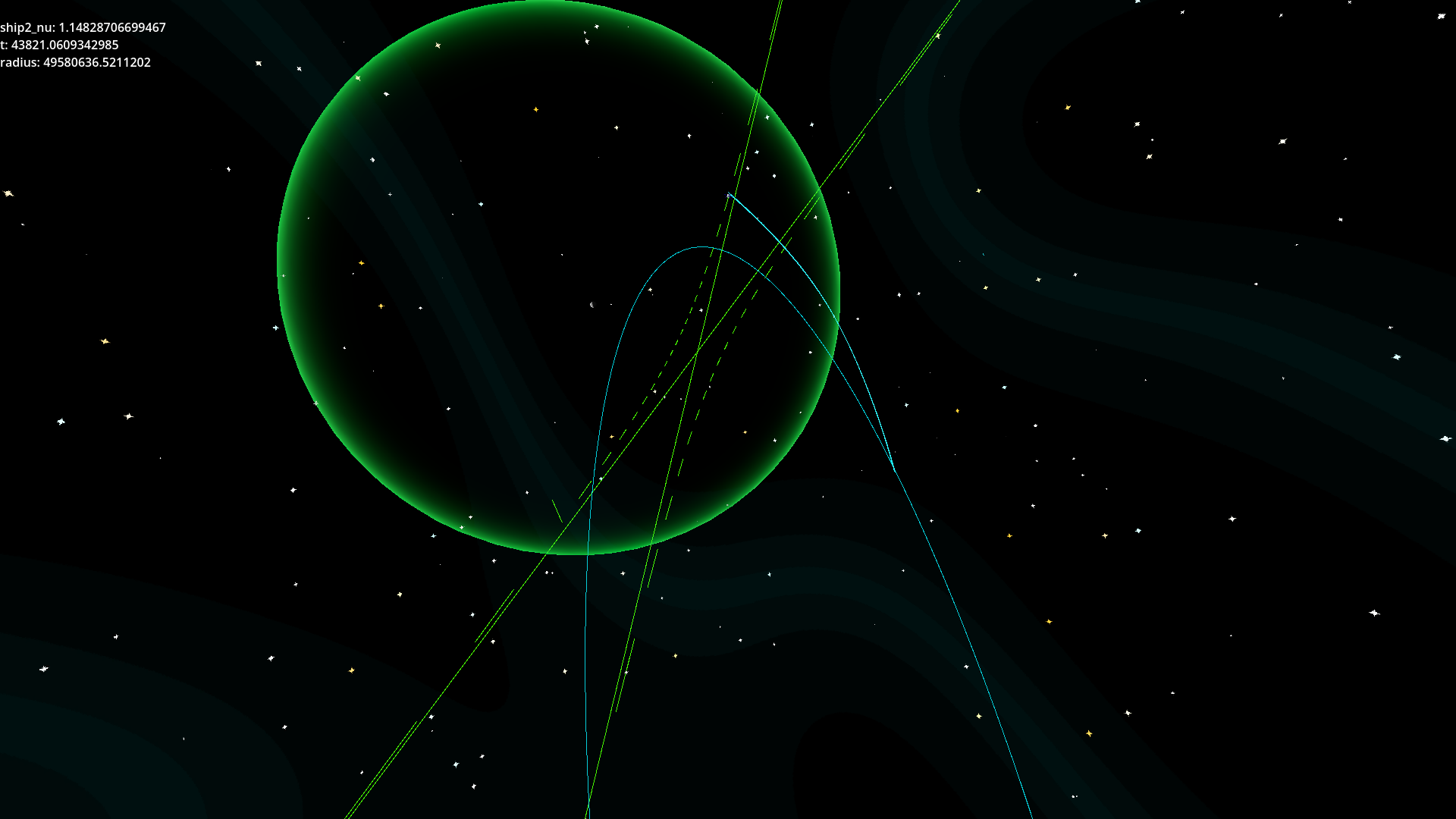
You will no doubt notice that when the ship crosses SOIs, it will deviate from its expected orbit as a function of the semi-major axis. This is more prominent in the Earth-Moon system as the Moon’s gravitational pull is significant even outside its SOI, and because of the steep angle when crossing into the SOI. This is an artifact inherent to patched conics. Compensating for it is an open question with multiple solutions. One such solution is the “Pseudostate Trajectory Model,” the gist of which is that it switches to the constrained 3-body problem some distance away from the SOI boundary, then back to 2-body physics once inside.

I didn’t want to learn the constrained 3-body problem just yet, so I tried using the Newtonian simulation in its place, which I saw referenced in another paper. This is, presumably, more computationally intensive, but easier to implement. For it to work, you need to compute the gravitational force vectors of both the planet and the moon while the spaceship crosses the SOI boundary. It’ll look a lot more “correct,” but at a cost.

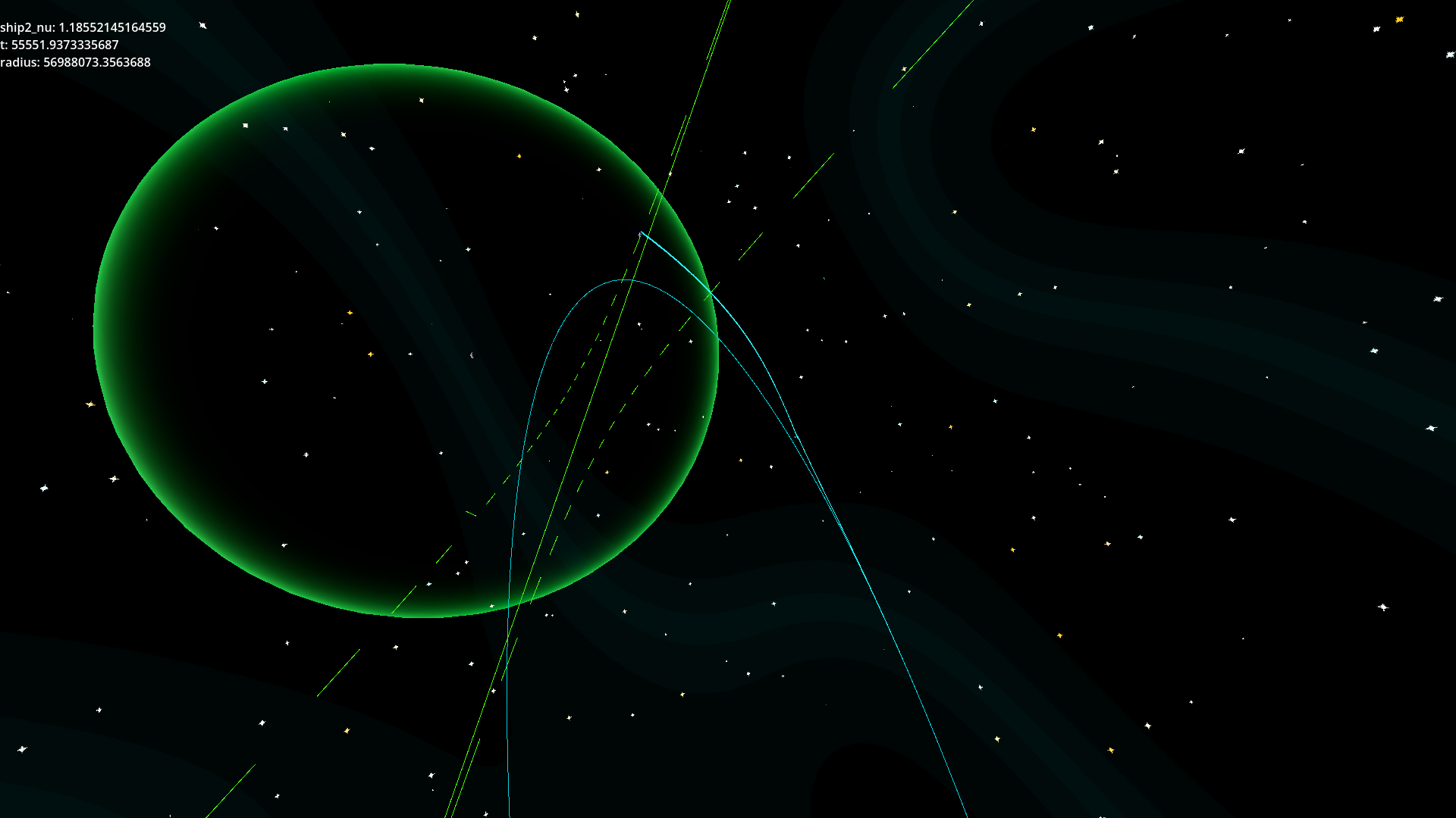
For my purposes, I did some tests and found that the difference in arrival time was only a few hours, so I’m probably going to skip it for Orbital Dawn. I might revisit the constrained 3-body problem later though.

I’m open to questions or comments, just bug me on social media!

-Silver